AI Doesn't See a BIM Model. AI Sees Data.

Why data distribution is one of the first concepts worth understanding in AI/ML

BIM is often associated with geometry.

We see a 3D building model, MEP systems, ducts, pipes, equipment, rooms, walls, slabs, and spatial relationships between elements. For a designer, BIM coordinator, or MEP engineer, the model is primarily a digital representation of the building.

But for artificial intelligence, a BIM model looks different.

For AI, a BIM model is not a “building”.

It is data.

pipe diameters,
duct lengths,
room areas,
air flow rates,
wall thicknesses,
system types,
clash counts,
family names,
IFC parameters,
element classes.

AI does not look at the model the way humans do. It does not see MEP systems as a logical layout until we transform them into a data structure it can learn from.

That is why, before we talk about training AI models for BIM, it is worth understanding a basic question:

How are our data distributed?

BIM as a dataset

Imagine a simple HVAC installation model.

For a human, it is a layout of ducts, supply diffusers, exhaust grilles, air handling units, dampers, and silencers. We can assess it visually, check routes, clashes, and design compliance.

For a machine learning algorithm, the same model can be a table:

Element	Length	Section	System	Flow	Level
Duct 1	1.2 m	400 × 200	Supply	350 m³/h	+3.20
Duct 2	2.4 m	500 × 250	Supply	620 m³/h	+3.20
Duct 3	0.8 m	315 mm	Exhaust	180 m³/h	+3.20
Duct 4	8.6 m	800 × 400	Supply	2200 m³/h	+3.20

Only at this level can AI start to “see” patterns.

It may notice that most ducts are short.
It may detect unusually large flow rates.
It may find elements with missing parameters.
It may recognise that certain element types often occur together.
It may help predict errors, classify elements, or optimise the design.

But for that to be possible, we first need to understand the language of data.

One of the most important concepts in that language is the data distribution.

What is a data distribution?

A data distribution describes which values appear in a dataset and how often they occur.

Example:

Suppose we analyse duct lengths in a BIM model.

We have values:

0.6 m
0.9 m
1.1 m
1.4 m
1.8 m
2.2 m
2.6 m
8.5 m
12.0 m

At first glance, most ducts are fairly short, but a few long segments also appear.

That is already information about the distribution.

We are not interested in a single average alone. We care about the shape of the data:

where values cluster,
how spread out they are,
whether outliers exist,
whether we have many small values and a few very large ones,
whether the data are uniform or highly skewed.

These questions matter enormously in machine learning.

Why the mean is not enough

In engineering work, we often like one concrete number.

Average duct length.
Average room area.
Average air flow.
Average number of clashes per storey.

The problem is that the mean can hide the true picture of the data.

Take this example:

1.0 m, 1.2 m, 1.4 m, 1.6 m, 12.0 m

The mean is:

3.44 m

But does a typical duct in this set measure about 3.4 m?

No.

Most ducts are about 1–2 m long. One long segment strongly inflated the mean.

That is why, in data analysis, we should look beyond the mean at the median, range, quartiles, standard deviation, and outliers.

In a BIM context this is especially important, because models often contain unusual cases:

very long mains,
very large rooms,
single elements with wrong units,
poorly defined families,
elements copied with incorrect parameters,
missing data in IFC.

For a human, that may be “one odd element”.

For an AI model, such an element can seriously disrupt training.

Probability mass — when data are discrete

Not all BIM data are continuous.

Sometimes we analyse values that are countable and appear as distinct cases.

Examples:

number of clashes per storey,
number of devices in a room,
number of diffusers in a zone,
number of IFC validation errors,
element class: wall, slab, roof, door,
system type: supply, exhaust, supply air, return air.

We call such data discrete.

For discrete data we can talk about the probability of a specific value.

For example:

P(X = 2)

meaning:

What is the probability that exactly 2 clashes occur on a given storey?

We call this approach probability mass.

Probability mass assigns a probability to specific values.

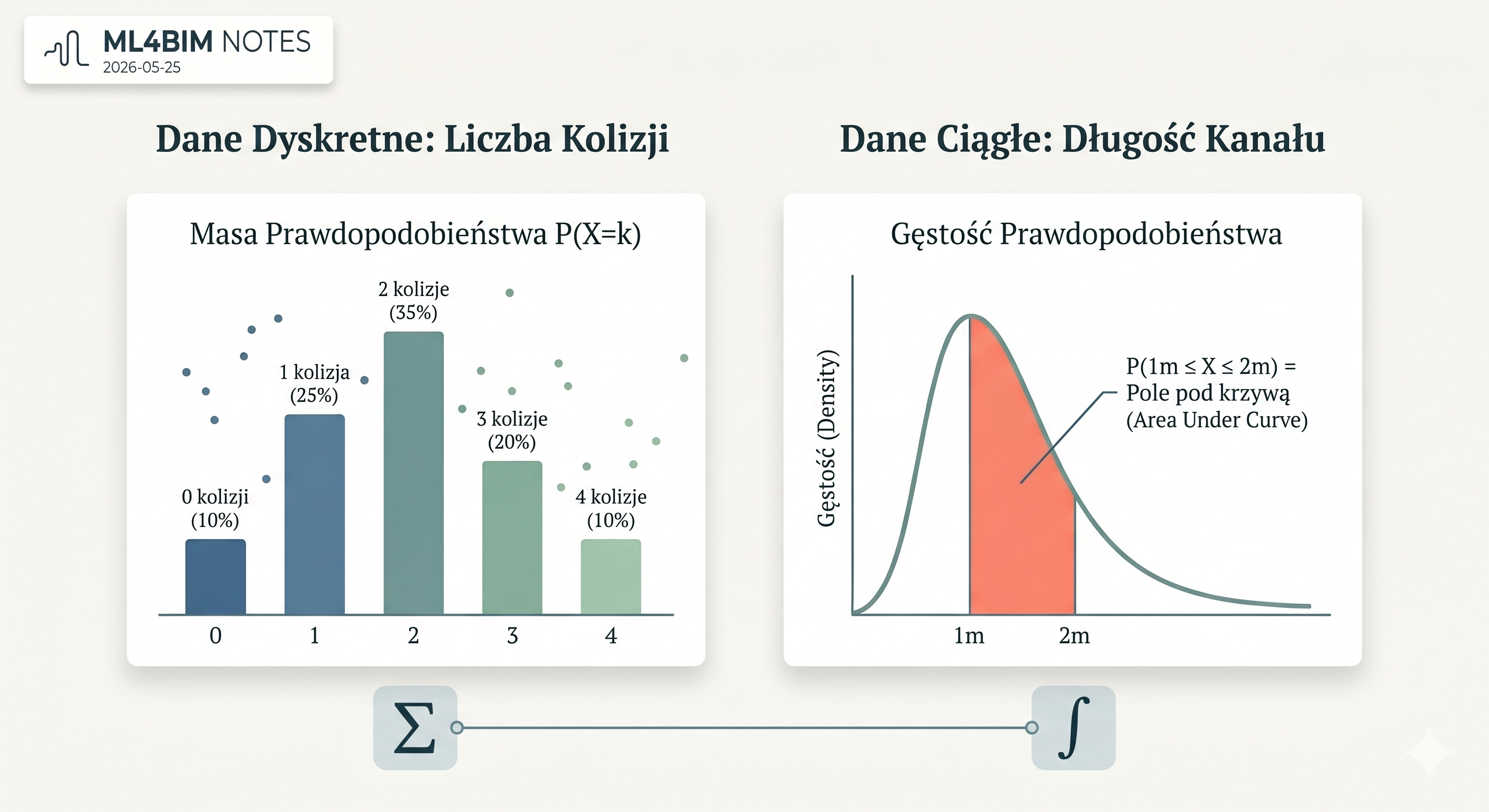
Example:

Number of clashes	Probability
0	10%
1	25%
2	35%
3	20%
4	10%

In this case we can say:

P(X = 2) = 35%

So there is a 35% probability that a given storey will have exactly two clashes.

That is intuitive, because the number of clashes can be 0, 1, 2, 3, and so on — distinct, separate values.

Probability density — when data are continuous

Continuous data work differently.

Continuous data can take any value within a range.

Examples from BIM and MEP:

duct length,
pipe diameter,
room area,
air flow rate,
temperature,
air velocity,
pressure drop,
partition thickness.

Here, asking for an exact value often makes little sense.

For example:

What is the probability that a duct is exactly 1.473829 m long?

In practice, such a question is not useful.

A duct length can take infinitely many possible values:

1.4 m
1.47 m
1.473 m
1.4738 m
1.47382 m
...

So for continuous data we usually do not ask about an exact value.

We ask about an interval.

For example:

What is the probability that duct length falls between 1 m and 2 m?

Here we introduce probability density.

Probability density tells us where values are more concentrated. If the density curve is high in a region, many values appear there.

But the height of the curve alone is not yet a probability.

Probability is the area under the curve over a given range.

Integration without scary mathematics

This is where integration comes in.

For many people, that sounds like difficult university maths. The intuition is much simpler.

In this context, integration means calculating the area under a curve.

If we have a probability density curve for duct lengths, the probability that a duct is between 1 m and 2 m long equals the area under the curve between 1 and 2.

You can picture it like this:

We have a curve describing the distribution of duct lengths.
We pick a range, e.g. from 1 m to 2 m.
We highlight the area under the curve in that range.
The area of that region is the probability.

In other words:

Probability = area under the curve

Integration is the mathematical way to compute that area.

That intuition matters, because many ideas in machine learning and statistics rely on this relationship.

Sum or integral?

The simplest way to remember:

For discrete data, we sum probabilities.

Example:

P(X = 1) + P(X = 2) + P(X = 3)

For continuous data, we compute the area under the curve — we use integration.

Example:

P(1 ≤ X ≤ 2)

Meaning:

the probability that the value falls between 1 and 2

In intuitive terms:

summing = adding separate bars
integration = adding very many thin slices under the curve

This is where mathematics starts to make practical sense for an engineer.

It is not about formulas for their own sake.

It is about understanding how an AI/ML model interprets data and their distribution — the chart above shows both approaches side by side.

Example: HVAC duct lengths

Suppose we want to train an AI model to recognise unusual elements in an HVAC installation.

One input feature might be duct length.

After analysing the data, we find:

most ducts are between 0.5 m and 3 m,
some ducts are between 3 m and 6 m,
a few ducts are longer than 10 m.

That tells us something important.

A 2 m duct is typical.
A 5 m duct is less typical but still plausible.
A 30 m duct may be a special case or a model error.

If we plot this distribution as a histogram, we will probably see many values on the left and a long tail on the right.

That means the data are skewed.

For AI this matters, because the model may learn typical cases very well but struggle with rare, unusual elements.

Data distribution and AI model quality

In machine learning, it is easy to get excited about the model itself.

Neural network.
Regression.
Classifier.
Language model.
AI agent.

But model quality often depends on something less flashy:

The quality and distribution of the input data.

If data are poorly described, the model learns wrong patterns.

If one class dominates, the model may ignore rare cases.

If outliers are not checked, they can distort predictions.

If units are inconsistent, the model may learn chaos.

If training data come from only one project type, the model may fail on other buildings.

In AEC this is especially important, because project data are often very uneven.

One model may have well-filled parameters.
Another may have gaps.
A third may use different naming.
A fourth may have a faulty IFC export.

AI does not automatically fix these problems. It inherits them.

That is why data analysis is the first step toward a sensible ML model.

What should an engineer check before training?

Before training an AI/ML model on BIM data, ask a few simple questions:

Which values occur most often?
Are there outliers?
Are the data discrete or continuous?
Are classes balanced?
Are there missing values?
Are units consistent?
Does the data distribution match project reality?
Do the data come from sufficiently diverse projects?

These are not academic questions.

They are practical ones.

If we want to classify building elements, we need to know which types dominate in the data.

If we want to analyse HVAC systems, we need to know how flows, diameters, lengths, and system types are distributed.

If we want to detect errors in an IFC model, we need to know what a “normal” model looks like before we detect anomalies.

The key intuition

BIM is geometry for humans.

For artificial intelligence, BIM is a dataset.

And data have a distribution.

The distribution tells us what is typical, what is rare, what is suspicious, and what an AI model can learn.

For discrete data we work with probability mass.

For continuous data we work with probability density.

For discrete data we sum probabilities.

For continuous data we compute the area under the curve — we integrate.

Although it sounds mathematical, the practical intuition is simple:

AI does not learn from magic. AI learns from the distribution of data.

Summary

If we want to develop artificial intelligence for BIM, we cannot start only with AI models.

We must start with data.

Their quality.
Their structure.
Their distribution.
Their limitations.

Only then can machine learning models make sense.

In BIM and MEP projects, data are often chaotic, inconsistent, and dependent on the standards of a given office, project, or IFC export. That is not an insurmountable obstacle. It is reality we need to understand and organise.

That is why data literacy — the ability to read and understand data — will be one of the key skills of the future BIM engineer.

Because before BIM becomes truly intelligent, it must become measurable.

ML4BIM Note #01

This article explains why the concept of data distribution is essential for applying AI in BIM. Using MEP examples, it covers probability mass, probability density, and integration — without academic jargon, from a practising engineer’s perspective.