How Does a Neural Network Learn to Drive Through a Building? Optimisation with BIM Racer

Imagine a floor plan in Revit. We can see walls, columns and passages between rooms. We choose a starting point and a destination. A small robot sets off, approaches a doorway, turns and tries to continue.

On screen, we see movement. Behind the scenes, a neural network converts distances and the direction of the route into two numbers: steering and target speed. Its behaviour depends on weights and biases. Changing these parameters can make the robot avoid a column, stop before an obstacle or drive into a wall.

Training means searching for parameters that lead to better decisions according to a chosen criterion. Mathematically, this is an optimisation problem.

In the previous article on regression in BIM 5D, we fitted a function that predicts construction costs. Now we will move on to a function that controls movement. Our example is BIM Racer: an experimental add-in for Revit 2024, also being developed as a laboratory for learning the mathematics of neural networks.

1. From a BIM model to the robot’s observations

The network in BIM Racer receives a small vector of numbers. Before we can prepare it, the building geometry goes through several stages:

Geometry in Revit
        ↓
Section through walls and columns → 2D obstacle map
        ↓
Robot simulation → sensor distances and speed
        ↓
Neural network → steering and target speed
        ↓
New robot position → next observation

The map is generated at a selected height above the level. Door openings come from the wall geometry, while door leaves are ignored. In practice, we therefore simulate open passages.

When we select a destination, another element comes into play: the A* algorithm plans a route using the entire map. The network receives a local cue about a point on that route and controls the robot’s movement.

This division matters when interpreting the experiment. A* handles path planning, while the learned component handles control. A successful run depends on both components and on the quality of the map.

The current prototype’s map excludes MEP systems, furniture, stairs, shafts and linked models, among other things. A single section also does not describe obstacles over the robot’s full height. This is an educational environment with simplified geometry.

2. Which numbers describe the situation?

The basic exploration variant has six inputs: five sensor distances and speed. The goal-directed variant adds three pieces of navigation information:

Input	Meaning	Range
$s_1,\ldots,s_5$	Distances to obstacles divided by the sensor range	$[0,1]$
$v/v_{\max}$	Current speed as a fraction of maximum speed	$[0,1]$
$\sin\alpha$	One component of the direction to the route point relative to the robot	$[-1,1]$
$\cos\alpha$	The other component of that direction	$[-1,1]$
$\min(1,d/R)$	Distance to the route point, capped at range $R$	$[0,1]$

The symbol $d$ denotes the distance to the selected route point, which is not always the final destination. The program selects the farthest visible node on the stored route. This allows the cue to guide the robot through a doorway even when it temporarily needs to move away from the destination.

Why represent direction with two numbers? Angles close to $-\pi$ and $\pi$ describe almost the same direction, even though their numerical values differ considerably. The sine–cosine pair preserves continuity at the full-turn boundary.

Distance scaling also has a simple interpretation. With a sensor range of 5 m, an obstacle 2 m away gives:

$$s=\frac{2}{5}=0.4.$$

The network therefore operates on comparable scales. In MEP applications, features expressed in different units, such as lengths, flow rates and power ratings, require similar care. Here, we scale using known physical limits, rather than standardising using statistics calculated from a dataset.

3. A neuron: sum, bias and activation

A single neuron performs two operations. First, it calculates a weighted sum and adds a bias:

$$z=\sum_{i=1}^{n}w_i x_i+b.$$

It then passes the result through an activation function. In BIM Racer, this is the hyperbolic tangent:

$$a=\tanh(z).$$

The inputs $x_i$ describe the current situation. The weights $w_i$ determine each signal’s contribution to the sum. The bias $b$ shifts that sum independently of the input values.

Suppose one input is $0.4$, its weight is $0.5$, and the remaining terms together with the bias add up to $0.1$. Then:

$$z=0.5\cdot0.4+0.1=0.3, \qquad a=\tanh(0.3)\approx0.2913.$$

If we increase only that weight to $1.0$, we get $z=0.5$ and an activation of approximately $0.4621$. We have changed the neuron’s response to the same observation. The eventual change in steering still depends on the connections further downstream.

The activation makes the network nonlinear. If every layer performed only linear operations with an added bias, their composition would still be a single affine function. Additional layers would not provide the same flexibility in describing relationships.

It is also useful to separate two issues: the ability to represent a complex function and the ability to find good weights. Universal approximation theorems address the former, under specific assumptions and with a sufficiently large network. They do not guarantee that a small robot controller will learn to drive without errors.

4. The entire network fits into two equations

The default navigation model has a 9 → 8 → 2 architecture: nine inputs, eight hidden neurons and two outputs.

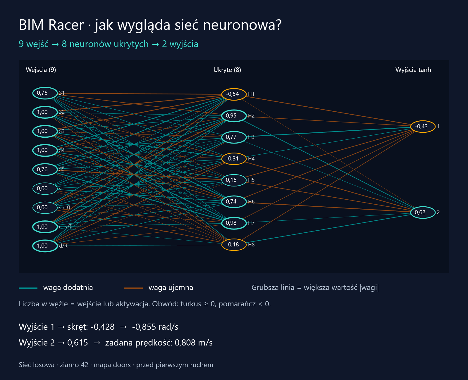
Figure 1. A diagram generated by the same component that draws the network in the “Brain” (“Mózg”) tab in Revit. It shows an untrained random network with seed 42 on the “doors” demo map, before the first movement. All numbers come from actual model calculations. The original labels are in Polish and decimal commas are used; the legend is explained in English below.

Read the diagram from left to right:

• Inputs: five sensors S1–S5, normalised speed v and the route cue: sin θ, cos θ and d/R. The symbol θ in the panel denotes the angle referred to as $\alpha$ in this article; d/R is a shortened label for $\min(1,d/R)$.
• Hidden layer: neurons H1–H8. Each receives all nine inputs. The number inside each neuron is the result of its tanh activation.
• Outputs: neuron 1 determines steering, while neuron 2 produces the value converted into target speed. Each uses all eight hidden neurons.
• Connections and outlines: a turquoise line indicates a positive weight, while an orange-brown line indicates a negative one; thicker lines correspond to larger absolute weights. The colour of a node’s outline indicates the sign of its input or activation: turquoise for non-negative values and orange for negative values.

The figure shows 88 connections: $9\cdot8+8\cdot2$. The remaining 10 parameters are the biases of the eight hidden neurons and the two output neurons; they do not have separate nodes in this diagram. The lines represent weights, rather than the current products of weights and signals, which is why they remain visible even when an input is zero.

For the observation shown, the network returns steering of approximately −0.428 and a second output of approximately 0.615. After scaling, this gives a target speed of about 0.808 m/s. This is a proposal from an untrained model, rather than an example of a correct navigation decision. In Revit, clicking a neuron expands its calculations; the illustration in this article is static.

We can express the same diagram using two equations:

$$\mathbf{h}=\tanh(W_1\mathbf{x}+\mathbf{b}_1),$$ $$\mathbf{y}=\tanh(W_2\mathbf{h}+\mathbf{b}_2).$$

The function $\tanh$ acts separately on each element of the vector. Matrix $W_1$ has dimensions $8\times9$, while $W_2$ has dimensions $2\times8$. Each neuron has its own bias, so the number of parameters is:

$$8\cdot9+8+2\cdot8+2=98.$$

These are 98 numbers that we can change during training. The 6 → 8 → 2 exploration variant has 74. The number of hidden neurons is configurable, so the network size may differ.

The outputs are converted into movement as follows:

$$u_{\mathrm{steering}}=y_1, \qquad v_{\mathrm{target}}=\frac{y_2+1}{2}\,v_{\max}.$$

The first number specifies normalised angular velocity. The second becomes the target linear speed. For example, $y_2=0.2$ means a speed of $0.6v_{\max}$. In this motion model, it is not an acceleration command.

During a run with a selected model, the weights remain fixed. The observations and the decisions derived from them change. This is inference: using an already prepared function. Training is a separate process in which we change its parameters.

4.1. Worked example: reading the inputs from the diagram

Let us trace one decision made by the exact network shown in Figure 1. We will first calculate the activation of neuron H1, then both control outputs. We use the recorded inputs, weights and biases of the untrained model with seed 42.

In the order shown on the left of the diagram, the inputs are:

$$\mathbf{x}= \begin{bmatrix} 0.76 & 1 & 1 & 1 & 0.76 & 0 & 0 & 1 & 1 \end{bmatrix}^{T}.$$

The superscript $T$ denotes transposition: the numbers displayed in one row form a column vector. The value $0.76$ for S1 means an obstacle at a distance of $0.76\cdot5=3.8$ m with a sensor range of 5 m. The speed input is zero because the robot has not yet moved. The pair $\sin\alpha=0$, $\cos\alpha=1$ indicates a route point directly ahead of the robot. The final 1 means that the distance to that point has reached or exceeded the range used for scaling; the input is capped at 1.

Numbers in the tables are rounded to six decimal places. Final results were calculated using the full precision of the data. The diagram displays activations to two decimal places, so small differences when calculating with the displayed values are to be expected.

4.2. Calculating neuron H1: multiply, sum and add the bias

H1 receives all nine inputs. It has a separate weight for each one. The first row of matrix $W_1$ contains these nine weights:

Input	Value $x_i$	Weight $w_{1i}$	Contribution to the sum $w_{1i}x_i$
S1	0.760000	−0.935957	−0.711328
S2	1.000000	−0.941454	−0.941454
S3	1.000000	−0.903868	−0.903868
S4	1.000000	0.690490	0.690490
S5	0.760000	0.614015	0.466651
Speed $v/v_{\max}$	0.000000	0.039987	0.000000
$\sin\alpha$	0.000000	0.651257	0.000000
$\cos\alpha$	1.000000	−0.738704	−0.738704
$\min(1,d/R)$	1.000000	0.587609	0.587609

For example, the connection S1 → H1 contributes:

$$w_{11}x_1\approx-0.935957\cdot0.76\approx-0.711328.$$

This connection has a negative weight, so a positive input reduces the neuron’s sum. Two other connections contribute zero in this observation: the current speed and the sine of the angle are both zero. Their weights still exist, but we multiply them by zero.

Adding all nine products gives approximately −1.550603. We then add H1’s bias, which is approximately 0.950429:

$$z_{H1}=\sum_{i=1}^{9}w_{1i}x_i+b_{H1} \approx-1.550603+0.950429 =-0.600174.$$

The bias is a separate additive term. In this example, it shifts the sum towards positive values, but it is not large enough to change its sign.

Now we apply the activation function:

$$h_1=\tanh(z_{H1}) \approx\tanh(-0.600174) \approx-0.537174.$$

This is the value −0.54 inside H1 in the diagram. A negative activation is a valid calculation result; it does not indicate an error or a “bad” neuron. It becomes an input signal for the next layer.

4.3. From eight activations to two outputs

Neurons H2–H8 follow the same procedure, each with its own nine weights and bias. We obtain eight activations. Both output neurons use all eight, but assign different weights to them.

In the table, $w^{(2)}_{1j}$ denotes the weight of the connection Hj → output 1, while $w^{(2)}_{2j}$ denotes the weight of Hj → output 2:

Neuron	Activation $h_j$	Weight to output 1	Contribution to output 1	Weight to output 2	Contribution to output 2
H1	−0.537174	−0.811879	0.436120	−0.049622	0.026656
H2	0.953364	−0.562832	−0.536583	0.655370	0.624806
H3	0.769621	0.990869	0.762593	0.118333	0.091072
H4	−0.306800	0.307405	−0.094312	−0.766471	0.235154
H5	0.156485	−0.674667	−0.105575	−0.595505	−0.093187
H6	0.744350	−0.642310	−0.478103	−0.893133	−0.664804
H7	0.983968	−0.371303	−0.365350	0.163804	0.161178
H8	−0.183059	−0.487592	0.089258	0.679734	−0.124431

Notice H1 and output 1. A negative activation multiplied by a negative weight gives a positive contribution of approximately 0.436120. An orange connection in the diagram therefore does not necessarily reduce the sum; its effect also depends on the sign of the signal it carries.

For the steering output, the sum of the eight contributions is approximately −0.291952. This output’s bias is approximately −0.165126:

$$z_{y_1}=\sum_{j=1}^{8}w^{(2)}_{1j}h_j+b^{(2)}_1 \approx-0.291952-0.165126 =-0.457078,$$ $$y_1=\tanh(z_{y_1})\approx-0.427700.$$

For the speed output, the contributions sum to approximately 0.256443, and the bias is approximately 0.461083:

$$z_{y_2}=\sum_{j=1}^{8}w^{(2)}_{2j}h_j+b^{(2)}_2 \approx0.256443+0.461083 =0.717526,$$ $$y_2=\tanh(z_{y_2})\approx0.615374.$$

We have now reproduced −0.43 and 0.62, the values shown in the two rightmost nodes of the diagram.

4.4. Converting the result into a movement command

In this example’s configuration, the maximum angular velocity is 2 rad/s and the maximum linear speed is 1 m/s. We therefore convert normalised steering as follows:

$$\omega_{\mathrm{target}}=y_1\omega_{\max} \approx-0.427700\cdot2 \approx-0.855399\ \mathrm{rad/s}.$$

The sign determines the direction of rotation according to the simulation’s coordinate system. The second output must first be rescaled from the interval −1 to 1 to the interval 0 to 1:

$$v_{\mathrm{target}}=\frac{y_2+1}{2}\,v_{\max} \approx\frac{0.615374+1}{2}\cdot1 \approx0.807687\ \mathrm{m/s}.$$

The network therefore proposes turning and moving at approximately 0.808 m/s at the same time. This is a control command issued before the simulation step. Only then will the simulation engine calculate movement and check for a collision. The current speed at the input is still zero; it describes the state before this decision.

4.5. What changes if we increase one weight by 0.1?

Finally, let us work through the numerical equivalent of a slider in the “Brain” panel. We change only the S1 → H1 weight, from approximately −0.935957 to −0.835957. All inputs, biases and other weights remain fixed.

The change in H1’s sum is:

$$\Delta z_{H1}=\Delta w_{11}\,x_1 =0.1\cdot0.76=0.076.$$

The new sum is approximately −0.524174, and the new activation is:

$$h'_1=\tanh(-0.524174)\approx-0.480915.$$

H1’s activation has increased by approximately 0.056258. The other hidden neurons’ activations have not changed, because we have not changed any of their inputs or parameters. In the output layer, we therefore only need to recalculate H1’s contribution:

$$z'_{y_1}=z_{y_1}+w^{(2)}_{11}(h'_1-h_1), \qquad z'_{y_2}=z_{y_2}+w^{(2)}_{21}(h'_1-h_1).$$

After applying tanh again and rescaling speed, we obtain:

Quantity	Original model	Copy with one weight changed
H1 sum	−0.600174	−0.524174
H1 activation	−0.537174	−0.480915
Normalised steering $y_1$	−0.427700	−0.464279
Target speed [m/s]	0.807687	0.806818

The increase in H1’s activation made steering more negative because the H1 → output 1 connection has a negative weight. The direction of change in a single parameter therefore does not translate directly into the direction of change in every output.

This calculation shows a behavioural change for one observation. To establish whether the new weight improves driving, we would need to evaluate runs of the modified model. In the experimental panel, we inspect only a copy of the decision; no movement is executed. We will discuss the relationship between parameter changes and the evaluation function below, with a separate example of a gradient step in Section 7.

5. What counts as good driving?

In regression, we compared a prediction with the actual value. In the current BIM Racer, we evaluate the outcome of an entire run using a fitness function. A higher value means a better result under the chosen scoring scheme.

With the default penalties, fitness for goal-directed navigation is:

$$F=100p+300g-0.5t-150c-2t_{\mathrm{stationary}}.$$

Here, $p$ denotes progress along the route in the range 0 to 1, $g$ is 1 when the destination has been reached, and $c$ is 1 after a collision. Run time $t$ and time spent stationary are measured in seconds. A collision ends the attempt.

Progress is based on the greatest reduction achieved so far in the remaining route length relative to its initial value. Revisiting the same sections does not allow the robot to collect the same reward repeatedly. If the destination has already been reached at the start, the progress term is zero.

The following numbers are a worked example, rather than measured model performance. We assume no time spent stationary:

Outcome	Assumptions	Fitness
Destination reached	$p=1$, $g=1$, $t=18$, $c=0$	$100+300-9=391$
Collision partway along the route	$p=0.6$, $g=0$, $t=8$, $c=1$	$60-4-150=-94$

Exploration mode uses a different scoring scheme: new cells and rooms are rewarded, while collisions, stationary time and time without discovering new cells are penalised. Once a destination is selected, exploration rewards are disabled. Defining the task changes the definition of success.

The evaluation function is part of the engineering design. If we rewarded only distance travelled, driving in circles might be beneficial. Without a reward for arrival, the robot might improve its partial score without completing the task.

For network parameters grouped together as $\theta$, we seek a high $F(\theta)$. Equivalently, we can define a loss $L(\theta)=-F(\theta)$ and seek its minimum. Simply changing the sign, however, does not give us a function suitable for direct differentiation through the entire simulation.

6. The gradient suggests how to change the parameters

One optimisation method is gradient descent:

$$\theta_{k+1}=\theta_k-\eta\nabla_\theta L(\theta_k).$$

The gradient contains the derivatives of the loss with respect to the parameters. It points in the direction of the steepest local increase in the loss under the standard geometry of parameter space. By subtracting a multiple of it, we try to reduce the loss. The positive learning rate $\eta$ determines the step size.

A small step may mean slow progress. Too large a step can worsen the result or destabilise training. A network’s loss surface is usually non-convex: it may contain local minima, saddle points and flat regions. A single direction of local improvement does not guarantee that we will find the best solution.

When training on a large set of examples, we often estimate the gradient using randomly selected small batches of data. This is how popular variants of stochastic gradient descent, or SGD, work. An update costs less than processing the entire dataset, but successive estimates of the direction can fluctuate. These mechanisms are discussed in more detail in the optimisation chapter of Deep Learning.

What might this kind of training look like for a robot? We could collect observations and the corresponding decisions made by a good controller, then minimise the imitation error. This is a possible direction for BIM Racer’s development; its current training uses a different method.

7. Backpropagation: calculating one step

Backpropagation calculates the gradient using the chain rule. The optimiser then uses that gradient to change the parameters. These are two separate tasks. This distinction is also visible in the PyTorch automatic differentiation documentation.

Consider a simplified example of a single neuron controlling steering:

$$\hat{u}=\tanh(wx+b), \qquad L=\frac{1}{2}(\hat{u}-u^*)^2.$$

The value $u^*$ denotes the desired steering supplied by a teacher. Let $x=0.4$, $w=0.5$, $b=0.1$ and $u^*=0.6$. This is a mathematical demonstration, rather than a record of BIM Racer training.

From our earlier calculation, we know that $\hat{u}\approx0.2913$. The loss is approximately $0.04764$. The chain rule gives:

$$\frac{\partial L}{\partial w} =\underbrace{(\hat{u}-u^*)}_{\text{effect of output on loss}} \underbrace{(1-\hat{u}^2)}_{\text{derivative of tanh}} \underbrace{x}_{\text{effect of weight on sum}} \approx-0.1130.$$

For the bias, the last factor is 1, so:

$$\frac{\partial L}{\partial b} =(\hat{u}-u^*)(1-\hat{u}^2) \approx-0.2825.$$

With $\eta=0.1$, updating both parameters using the same initial values gives:

$$w_{\mathrm{new}}\approx0.5113, \qquad b_{\mathrm{new}}\approx0.12825.$$

The new output is approximately $0.3210$, and the loss falls to $0.03892$. This step has moved us closer to the desired steering.

In a multilayer network, the calculation involves more dependencies. Backpropagation traverses the computational graph from the loss towards the earlier layers and reuses intermediate results. This makes it possible to calculate the effect of every weight without changing each one separately and repeating the entire experiment.

8. How does BIM Racer actually train?

The current implementation selects weights using a genetic algorithm. This way of training a network is called neuroevolution. Evaluation comes from simulated runs, while new parameters are produced through selection, crossover and mutation.

One generation proceeds as follows:

1. Each network in the population controls the robot in the specified scenarios.
2. The program calculates each network’s fitness. For navigation, this is the mean score across all training scenarios.
3. The best individuals pass unchanged into the next generation; this is elitism.
4. Parents of the remaining individuals are selected through tournaments of three networks.
5. Each offspring parameter is randomly inherited from one of the two parents.
6. Selected parameters receive a random mutation. This produces a new population to evaluate.

The default settings include a population of 64 networks, 6 retained elites, a mutation probability of 0.05 for each parameter and a mutation strength of 0.2. A mutation adds a Gaussian perturbation with a standard deviation of 0.2 to the parameter. Offspring parameters are clipped to the interval −10 to 10.

The navigation variant evaluates each network on nine scenarios: the current map and eight synthetic maps. The entire population uses the same set, allowing results to be compared.

This approach does not require calculating derivatives through collisions, route-point selection or episode termination. The cost is having to run many simulations. The network itself, with its tanh activation, is differentiable, but the current training process does not differentiate through the entire run-evaluation mechanism.

Element	Gradient-based learning in the demonstration	Neuroevolution in this example
Quality signal	Error relative to the teacher’s decision	Run score
How weights change	Gradient-based update	Crossover and mutation
Main setting controlling change size	Learning rate	Mutation strength
Unit of progress	Parameter update after a batch of data	Population evaluation and reproduction
Backpropagation	Used to calculate the gradient	Not performed

The table compares two specific approaches to this project. Gradient-based methods can also learn from rewards, for example in policy gradient algorithms; they are not limited to imitating a teacher.

9. Initialisation and saturation affect network behaviour

Training begins with an initial set of weights. In BIM Racer, the initial population uses random sampling that depends on the layer’s input and output counts:

$$w\sim U\left(-\sqrt{\frac{6}{n_{\mathrm{in}}+n_{\mathrm{out}}}}, \sqrt{\frac{6}{n_{\mathrm{in}}+n_{\mathrm{out}}}}\right).$$

Biases are initially zero. This is Glorot initialisation, also known as Xavier initialisation. The importance of the scale of initial weights is described in the paper by Glorot and Bengio. The project’s educational “Random network” (“Sieć losowa”) button uses a simpler parameter-sampling method; it should not be confused with the initialisation of the training population.

Why does scale matter? For a large positive sum $z$, $\tanh(z)$ approaches 1, while for a large negative sum it approaches −1. The neuron is then saturated. Further changes in the sum may produce only a small change in activation.

With gradient-based learning, this appears in the derivative $1-\tanh^2(z)$, which becomes small. In our evolutionary training, the effect is different: a mutation may change a weight while barely changing the decision. In both cases, it is useful to inspect the calculations, rather than just parameter magnitudes.

Parameters and hyperparameters play different roles. Parameters are the weights and biases selected during training. Hyperparameters describe the learning process and model architecture, such as the number of neurons, population size or mutation strength. Reward and penalty coefficients, meanwhile, define the quality criterion itself. Increasing the population, enlarging the network and raising the collision penalty change three different parts of the experiment.

10. A good training result needs testing on new maps

The repository contains a recorded experiment with seed 42, a population of 32 networks, 20 generations and 12 hidden neurons. Each attempt was limited to 1,800 steps of 1/60 s, or 30 seconds. This was therefore a 9 → 12 → 2 model, larger than the default variant with eight neurons.

The report contains the following results:

Model and scenario set	Destinations reached	Collisions
Network — training	9/9	0
Network — six other test maps	5/6	1
A* + rule-based controller — the same test maps	6/6	0

The network reached every destination in the training scenarios, yet still made an error on one new map. A simple path-following controller was more effective in this small test. Both solutions used A* routes, so the comparison primarily concerns motion control.

The best-fitness chart in the training panel shows the best result found up to each generation. Under fixed conditions, this record does not decrease because the program preserves it. The population mean can fluctuate. Neither curve replaces evaluation on new maps.

A separate test in the project contains six layouts excluded from training, but they still come from a similar family of synthetic arrangements. Assessing transfer to practical BIM applications would require different, previously unseen buildings and repeated experiments with several random seeds.

When selecting settings, we also need to distinguish validation from the final test. If we keep improving the model after inspecting results on the same six maps, those maps start to serve as a validation set. Final evaluation then requires another, unused set.

11. Where does regularisation come in?

Regularisation helps limit overfitting to training data. Methods include penalties on weight magnitudes, dropout and early stopping.

An L2 penalty adds a term to the loss proportional to the sum of squared weights:

$$L_{\mathrm{reg}}=L_{\mathrm{task}}+\lambda\sum_j w_j^2.$$

The coefficient $\lambda\geq0$ sets the strength of the penalty relative to the task loss. An L1 penalty uses the sum $\sum_j|w_j|$ and favours sparse solutions in which some weights are zero. Dropout randomly sets some activations to zero during training. Early stopping ends training according to a chosen validation criterion when further training stops improving performance. These techniques are also described in the regularisation chapter of Deep Learning.

Batch normalisation normalises activations using training-batch statistics and learned transformation parameters. It can also affect generalisation, but it is a different mechanism from scaling our sensor readings by their range. It was described in the paper by Ioffe and Szegedy.

The current BIM Racer does not implement dropout, batch normalisation, L1/L2 penalties or automatic validation-based stopping. Clipping offspring parameters to the interval −10…10 constrains the search space; it is not an L2 penalty. Training on multiple maps increases the diversity of experience, but does not guarantee generalisation.

Before adding further techniques, a useful experiment would be to compare several network sizes on a separate validation set. More parameters increase both the model’s capacity and the space the algorithm has to search.

12. What does this experiment offer BIM and MEP engineers?

BIM Racer makes the full connection between geometry representation, observation, network computation and outcome evaluation visible. When the robot makes a mistake, we can inspect the numbers it received, how it transformed them and why points were awarded.

This approach to analysis also helps with other tasks: predicting energy consumption, building surrogate models for HVAC calculations or evaluating design alternatives. In each case, we need to define the inputs, the model function, the quality criterion and the conditions for testing it on new data.

It is useful to be precise about what is being optimised. In this experiment, we optimise controller parameters. The building geometry remains the test environment. Optimising ventilation duct routes would require a different representation of decisions, spatial constraints and evaluation criteria. That would be a separate task requiring its own design.

The most instructive moment in BIM Racer comes when we stop the robot before a doorway, change one weight and see the decision change. We can then trace the path from a number in a matrix to behaviour on a floor plan. And afterwards, we can test whether that behaviour actually leads to the destination in another building as well.

Sources and basis of the article

• Hala Nelson, Matematyka i sztuczna inteligencja. Kluczowe koncepcje zwiększania skuteczności i wydajności systemów, Chapter 4: “Optymalizacja w sieciach neuronowych” (Optimisation for Neural Networks), Helion, Polish edition. Publisher’s description and table of contents.
• Hala Nelson, Essential Math for AI, Chapter 4: “Optimization for Neural Networks”. O’Reilly public preview.
• Source code, MVP 4.3 documentation and the recorded experiment report for BIM Racer, as reviewed on 6 October 2026. Architecture settings, the training algorithm and run results come from the project.
• Ian Goodfellow, Yoshua Bengio, Aaron Courville, Deep Learning: optimisation and regularisation.
• Xavier Glorot, Yoshua Bengio, Understanding the difficulty of training deep feedforward neural networks, 2010.
• Sergey Ioffe, Christian Szegedy, Batch Normalization: Accelerating Deep Network Training by Reducing Internal Covariate Shift, 2015.
• PyTorch, Automatic Differentiation with torch.autograd.